How Image Edge Detection Works

4 min readSep 30, 2018

This week’s edition — edge detection in images. More specifically we’ll be taking a closer look at the Sobel Edge Detection algorithm.

Let’s start from the beginning.

Grayscale Images

The Sobel algorithm works by measuring the varying pixel intensity in an image. Naturally, this is easiest to accomplish when the image is a standardized grayscale image.

There are several algorithms to generate grayscale images — the simplest being an average of the R,G, and B values in a pixel.

Then, we re-assign these new intensity values to the R,G, and B fields of the original pixel. Any situation where all the R,G, and B values are the same will give you a shade of gray (remember #00000 is black and #FFFFFF is white).

However, though this often gives good results, the following grayscale function uses a weighted average that is better aligned with how the human eye interprets different colors and the transition between them.

Regardless of which formula we use, we now have a grayscale image that we can apply the Sobel Edge Detection algorithm too.

Sobel Detection Algorithm

The Sobel algorithm was developed by Irwin Sobel and Gary Feldman at the Stanford Artificial Intelligence Laboratory (SAIL) in 1968.

In the simplest terms, their algorithm works by running a 3x3 matrix (known as the kernel) over all the pixels in the image. At every iteration, we measure the change in the gradient of the pixels that fall within this 3x3 kernel. The greater the change in pixel intensity, the more significant the edge there is.

Convolution

The algorithm relies heavily on a mathematical operation called convolution.

Convolution is simply the process of multiplying and adding corresponding indices of two matrices together (the kernel and the image matrix) after flipping both the rows and the columns of the kernel.

The kernel on the left has its rows and columns flipped and then multiplied by the corresponding indices in the image matrix.

The standard implementation of the algorithm uses the following 3x3 matrices for the x and y axis, respectively.

Pre-Convoluted Kernel (A is a matrix containing the image data)

Now, we have completed all of the pre-processing and have the convoluted matrices in hand.

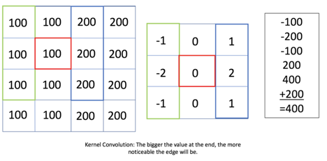
We can iterate through all pixels in the original image and apply the image convolution kernels Gx and Gy at every step of the way. This convolution operation will return a single integer for each kernel.

Here’s an example of what applying the Gx kernel on a specific pixel (in red) would look like:

On the left is the original image with the 3x3 pixel group colored

The penultimate step is to create a new image of the same dimensions as the original image and store for the pixel data, the magnitude of the two gradient values:

A recommended next step would be to normalize all of the data in the new image by dividing all the pixel values by the greatest gradient magnitude observed.

Now, you have a new grayscale image whose pixel intensities reflects how close they are to an edge in the original image. Naturally, the higher the gradient value for the pixel, the brighter the edge in the resultant image will appear.